L5: Performance of Parallel Systems

Performance Goals:

• Users: reduced response time → Time between the start and termination of the program
• Computer managers: high throughput
  • Average number of work units executed per unit time, e.g. jobs per second, transactions per second

Execution Time

Response Time in Sequential Programs (wall-clock time): includes

• User CPU time: time CPU spends for executing program
• System CPU time: time CPU spends executing OS routines
• Waiting time: I/O waiting time and the execution of other programs because of time sharing

Considerations:

• waiting time: depends on the load of the computer system
• system CPU time: depends on the OS implementation

User CPU Time

Depends on:

• Translation of program statements by the compiler into instructions

• Execution time for each instruction:

  $Time_{user}(A) = N_{cycle}(A) \times Time_{cycle}$

  • $Time_{user}$ → User CPU time of a program A
  • $N_{cycle}(A)$ → Total number of CPU cycles needed for all instructions
  • $Time_{cycle}$ → Cycle time of CPU (clock_cycle_time = 1/clock_rate)

But instructions may have different execution times

→ For a program with n types of instructions, I1,…, In

$$N_{cycle}(A) = \sum_{i = 1}^n {n_i(A)\times CPI_i}$$

• $n_i(A)$ → number of instructions of type Ii
• $CPI_i$ → average number of CPU cycles needed for instructions of type Ii

Thus:

$$Time_{user} = N_{instr}(A) \times CPI(A) \times Time_{cycle}$$

• $CPI(A)$ → depends on the internal organization of the CPU, memory system, and compiler
• $N_{instr}(A)$ → total number of instructions executed for A, depends on the architecture of the computer system and the compiler

Include memory access time to the user time:

$$Time_{user}(A) = \left(N_{cycle}(A) + N_{mm\_cycle}(A) \right) \times Time_{cycle}$$

• $N_{mm\_cycle}(A)$ → number of additional clock cycles due to memory accesses

Consider a one-level cache:

$$N_{mm\_cycle}(A) = N_{read\_cycle}(A) + N_{write\_cycle}(A) \\[10px] N_{read\_cycle}(A) = N_{read\_op}(A) \times R_{read\_miss}(A) \times N_{miss\_cycle}(A)$$

$N_{mm\_cycle}(A)$ is similar

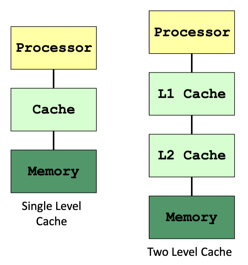
Memory Access: Illustration

Terminology:

• LLC = last level cache
• Cache line/block = each block of memory content in cache
• Mapping = mechanism used to store and locate a memory block in cache

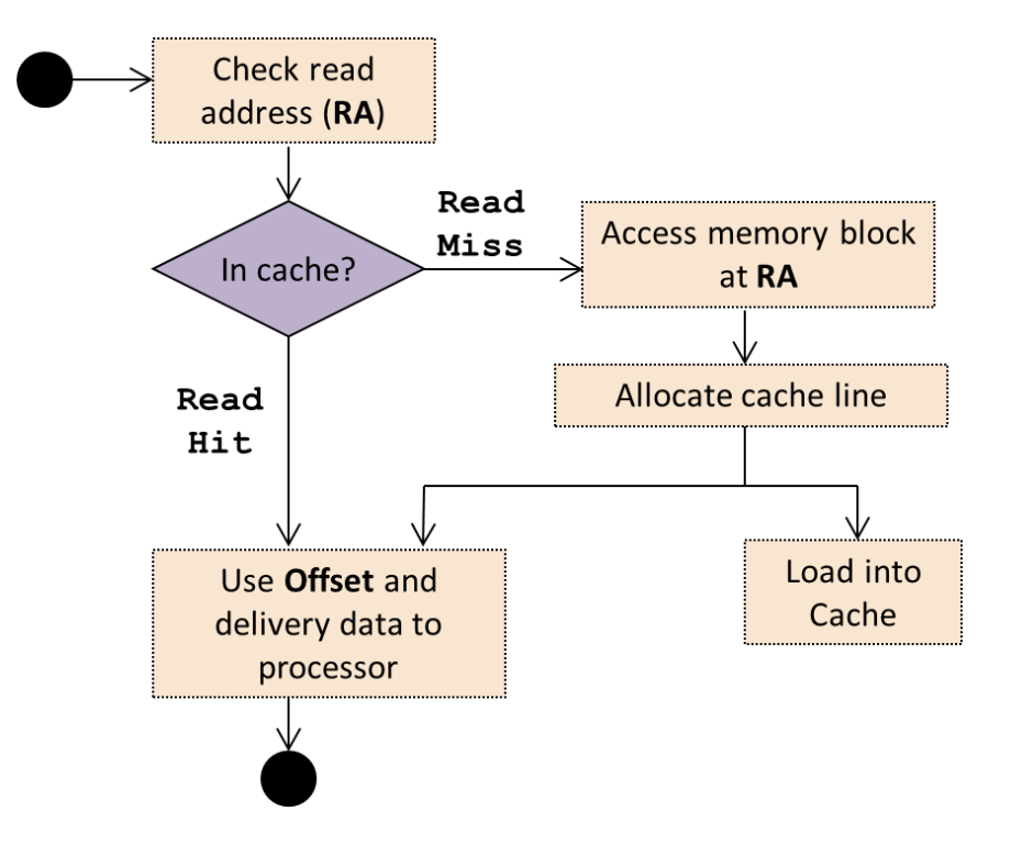
Read access (load) workflow

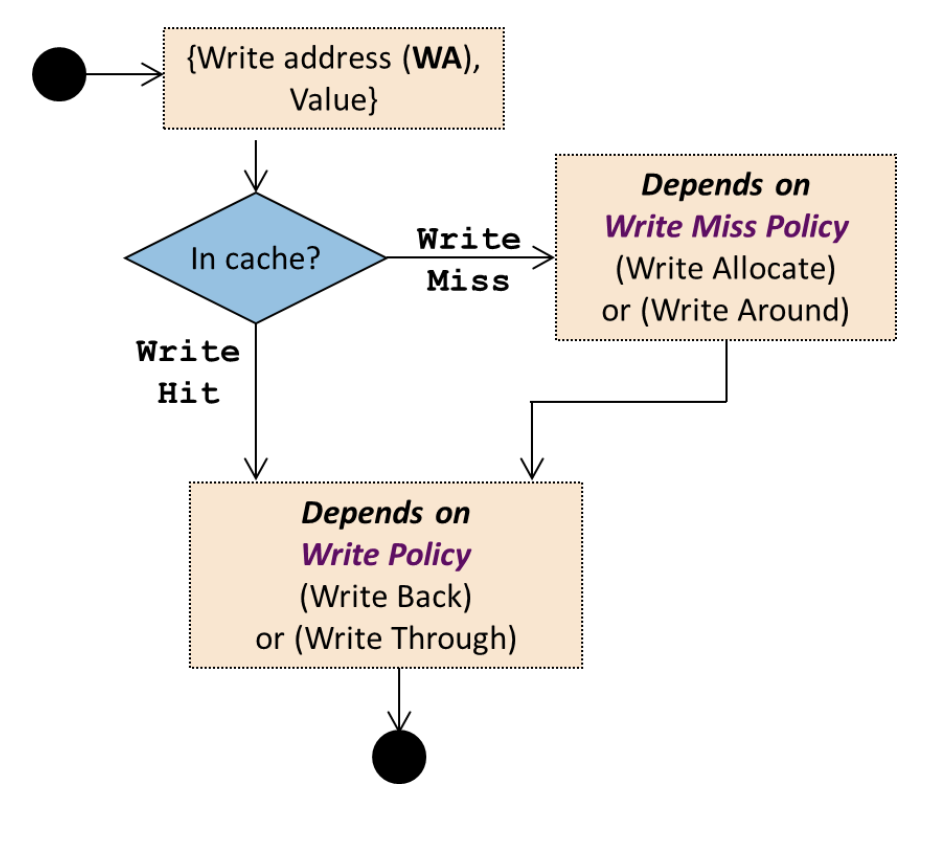
Write access (store) workflow

Refinement with Memory Access Time:

• User time with instructions with different execution times extension:

  $$Time_{user}(A) = \\ \left(N_{instr}(A) \times CPI(A) + N_{rw\_op}(A) \times R_{miss}(A) \times N_{miss\_cycles}(A) \right) \times Time_{cycle}$$
  • $N_{rw\_op}$ → total number of read or write operations
  • $R_{miss}(A)$ → (read and write) miss rate
  • $N_{miss\_cycles}$ → number of additional cycles needed for loading a new cache line

Average Memory Access Time:

$$T_{read\_access}(A) = T_{read\_hit} + R_{read\_miss}(A) \times T_{read\_miss}(A)$$

• $T_{read\_access}(A)$ → average read access time of a program A
• $T_{read\_hit}$ → time for a read access to the cache irrespective of hit or miss (additional time is captured in misses)
• $R_{read\_miss}(A)$ → cache read miss rate of a program A
• $T_{read\_miss}(A)$ → read miss penalty time
• Can be applied to multiple level of cache or virtual memory

$$T_{read\_access}(A) = T^{L1}*{read\_hit} + R^{L1}*{read\_miss}(A) \times T^{L1}*{read\_miss}(A) \\[10px] T^{L1}*{read\_miss}(A) = T^{L2}*{read\_hit} + R^{L2}*{read\_miss}(A) \times T^{L2}_{read\_miss}(A)$$

• Global miss rate: $R^{L1}*{read\_miss}(A) \times R^{L2}*{read\_miss}(A)$

Example:
Processor for which each instruction takes 2 cycles to execute. The processor uses a cache for which the loading of a cache block takes 100 cycles. Program A for which the (read and write) miss rate is 2% and in which 33% of the instructions executed are load and store operations

Scenarios – Execution time when

• No cache

$$Time_{user}(A) = \left(N_{cycle}(A) + N_{mm\_cycle}(A) \right) \times Time_{cycle} \\[10px] Time_{user}(A) = \left(N\times2 + 0.33N\times1\times100 \right) \times Time_{cycle} = 35 \frac{N}{f} \tag{1}$$

• Double clock rate while the time to load a cache block doubles (200 cycles)

$$Time_{user}(A) = \left(N\times2 + 0.33N\times0.02\times200 \right) \times Time_{cycle} = (3.32)\frac{N}{2f} \tag{2} \\[10px] \therefore \frac{(1)}{(2)} = \frac{35\times2}{3.32} = 21.08$$

→ Case (2) is 21.08 times more efficient than case (1)

Throughput

Million-Instruction-Per-Second:

$$MIPS(A) = \frac{N_{instr}(A)}{Time_{user}(A)\times 10^6} \\[10px] MIPS(A) = \frac{f}{CPI(A) \times 10^6}$$

• Drawbacks:
  • Consider only the number of instructions
  • Easily manipulated (by making instruction smaller)

Million-Floating point-Operation-Per-Second:

$$MFLOPS(A) = \frac{N_{fl\_ops}(A)}{Time_{user}(A)\times 10^6} \\[10px]$$

• $N_{fl\_ops}(A)$ → number of floating-point operations in program A
• Drawback: No differentiation between different types of floating-point operations

Speedup

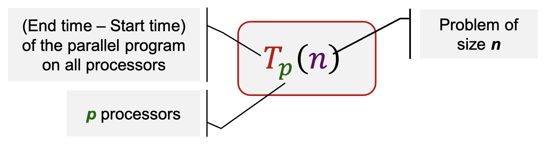
Parallel Execution Time

Consists of:

• Time for executing local computations
• Time for exchange of data between processors
• Time for synchronization between processors
• Waiting time
  • Unequal load distribution of the processors
  • Wait to access a shared data structure

Parallel Program: Cost

Cost of a parallel program with input size n executed on p processors:

$$C_p(n)= p\times T_p(n)$$

$C_p(n)$ measures the total amount of work performed by all processors, i.e. processor-runtime product

A parallel program is cost-optimal if it executes the same total number of operations as the fastest sequential program

Parallel Program: Speedup

• Measure the benefit of parallelism: a comparison between sequential and parallel execution time

$$S_p(n) = \frac{T_{best_seq}(n)}{T_p(n)} = \frac{T_\*(n)}{T_p(n)}$$

• Theoretically, $S_p(n) \leq p$ always holds
• In practice, $S_p(n) > p$ (superlinear speedup) can occur, for e.g. when problem working task “fits” in the cache

Best Sequential Algorithm:

• Best sequential algorithm may not be known
• There exists an algorithm with the optimum asymptotic execution time, but other algorithms lead to lower execution times in practice
• Complex implementation for the fastest algorithm

Parallel Program: Efficiency

Actual degree of speedup performance achieved compared to the maximum

$$E_p(n) = \frac{T_*(n)}{C_p(n)} = \frac{S_p(n)}{p} = \frac{T_*(n)}{p\times T_p(n)}$$

Ideal speedup: $S_p(n) = p \Rarr E_p(n) = 1$

Scalability

Interaction between the size of the problem and the size of the parallel computer

• Impact on load balancing, overhead, arithmetic intensity, locality of data access
• Application dependent

Fixed problem size and the machine

• Small problem size:
  • Parallelism overheads dominate parallelism benefits
  • Problem size may be appropriate for a small machine, but inappropriate for large one
• Large problem size: (problem size chosen to be appropriate for large machine)
  • Key working set may not “fit” in small machine (causing thrashing to disk, or key working set exceeds cache capacity, or can’t run at all)

Scaling Constraints:

• Application-oriented scaling properties (specific to application)
  • Particles per processor in a parallel N-body simulation
  • Transactions per processor in a distributed database
  • In practice, problem size is a combination of parameters, not only one number
• Resource-oriented scaling properties
  • Problem constrained scaling (PC): use a parallel computer to solve the same problem faster
  • Time constrained scaling (TC): completing more work in a fixed amount of time
  • Memory constrained scaling (MC): run the largest problem possible without overflowing main memory

Amdahl’s Law

Note

💡 Speedup of parallel execution is limited by the fraction of the algorithm that cannot be parallelized (f).

f (0 ≤ f ≤ 1) is called the sequential fraction Also known as fixed-workload performance

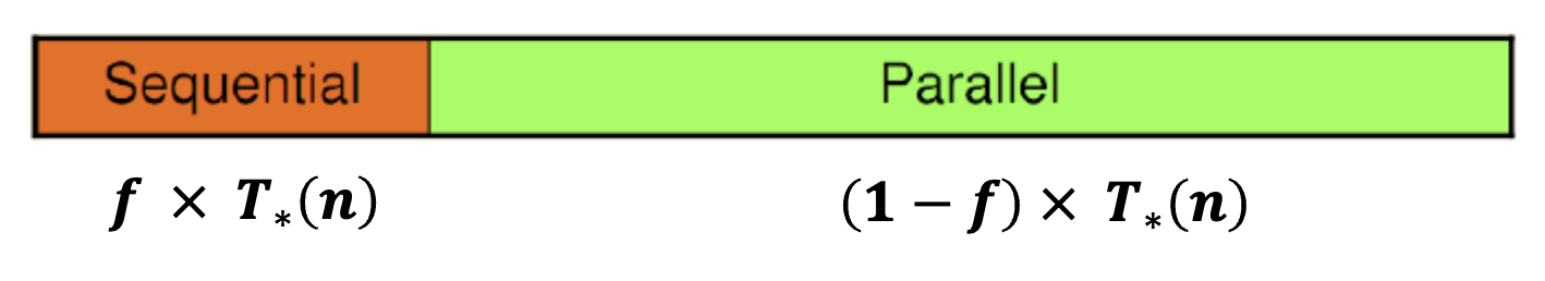
Sequential Execution Time

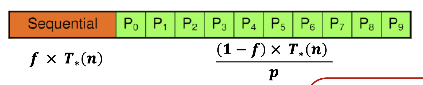
Parallel Execution Time

$$S_p(n) = \frac{T_*(n)}{f\times T_*(n) + \frac{1-f}{p}\times T_*(n)} = \frac{1}{f + \frac{1-f}{p}} \leq \frac{1}{f}$$

However, in many computing problems, f is not a constant

• Commonly dependent on problem size n
• f is a function of n, f(n)

An effective parallel algorithm is:

$$\lim_{x \to \infty} f(x) = 0$$

Thus, speedup:

$$\lim_{x \to \infty} S_p(n) = \frac{p}{1 + (p - 1)\ f(n)} = p$$

→ Amdahl’s Law can be circumvented for large problem size!

Gustafson’s Law (1988)

There are certain applications where the main constraint is execution time

• e.g. weather forecasting, chess program, etc
• Higher computing power is used to improve accuracy / better result

If f is not a constant but decreases when problem size increases, then $S_p(n) \leq p$

$\tau_f$ → constant execution time for sequential part

$\tau_\nu(n, p)$ → execution time of the parallelizable part for a problem of size n and p processors

$$S_p(n) = \frac{\tau_f + \tau_\nu(n, 1)}{\tau_f + \tau_\nu(n, p)}$$

Assume parallel program is perfectly parallelizable (without overheads), then

$$\tau_\nu(n, 1) = T_*(n) - \tau_f \text{ and } \tau_\nu(n, p) = \frac{T_*(n) - \tau_f}{p}$$

If T*(n) increases strongly monotonically with n, then $\lim_{x \to \infty} S_p(n) = p$

Communication Time

Message Transmission: Sender

Sending processor

To send a message

• Message is copied into a system buffer
• A checksum is computed
• A header is added to the message
• A timer is started and the message is sent out

After sending the message

• If acknowledgment message arrives, release the system buffer
• If the timer has elapsed, the message is re-sent
  • Restart timer, possibly with a longer time

Message Transmission: Receiver

Receiving processor

Message is copied from the network interface into a system buffer

Compare computed checksum and received checksum

• Mismatch: discard the message; re-sent after the sender timer has elapsed
• Identical: message is copied from the system buffer into the user buffer; application program gets a notification and can continue execution

Performance Measures

Measure	Definition	Unit
Bandwidth	Maximum rate at which data can be sent	bits (bytes) per second
Byte transfer time	Time to transmit a single byte	Seconds/byte
Time of flight	Time the first bit arrived at the receiver (channel propagation delay)	second
Transmission time	Time to transmit a message	second
Transport latency	Total time to transfer a message = transmission time + time of flight	second
Sender overhead	Time of computing the checksum, appending the header, and executing the routing algorithm	second
Receiver overhead	Time of checksum comparison and generation of an acknowledgment	second
Throughput	Effective bandwidth	bits (bytes) per second

Total Latency of a Message of Size m:

$$T(m) = O_{send} + T_{delay} + \frac{m}{B} + O_{recv} = T_{overhead} + \frac{m}{B} = T_{overhead} + t_B\times m$$

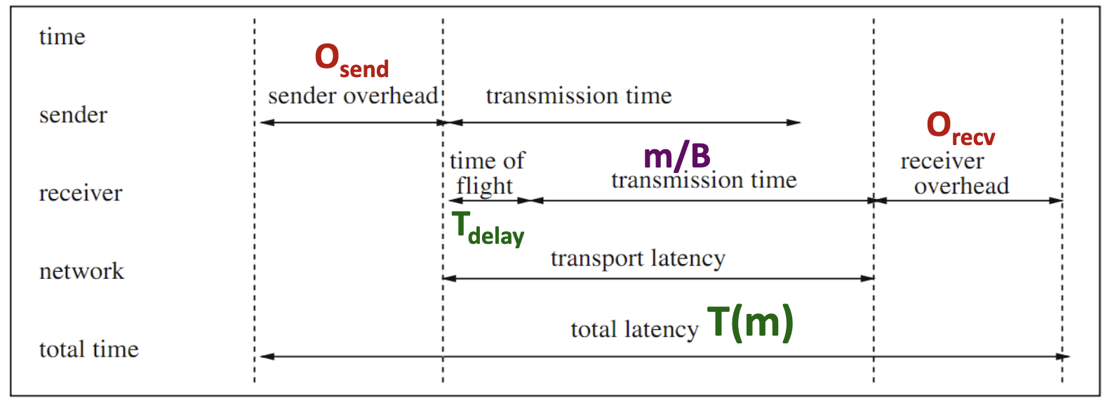
• $B$ → network bandwidth
• $T_{delay}$ → time first bit to arrive at receiver
• no checksum error and network contention and congestion,
• $T_{overhead} = O_{send} + T_{delay} + O_{recv}$ → is independent of the message size
• $t_B = \frac{1}{B}$ → the byte transfer time

Performance Analysis

Experimentation Challenges

Experiment with writing and tuning your own parallel programs

• Many times, we obtain misleading results or tune code for a workload that is not representative of real-world use cases

Start by setting your application performance goals

• Response time, throughput, speedup?
• Determine if your evaluation approach is consistent with these goals

Try the simplest parallel solution first and measure performance to see where you stand

Performance analysis strategy:

• Determine what limits performance:
  • Computation
  • Memory bandwidth (or memory latency)
  • Synchronization
• Establish the bottleneck

Possible bottlenecks

Instruction-rate limited: add “math” (non-memory instructions)

• Does execution time increase linearly with operation count as math is added?

Memory bottleneck: remove almost all math, but load same data

• How much does execution-time decrease?

Locality of data access: change all array accesses to A[0]

• How much faster does your code get?

Synchronization overhead: remove all atomic operations or locks

• How much faster does your code get? (provided it still does approximately the same amount of work)