Final notes

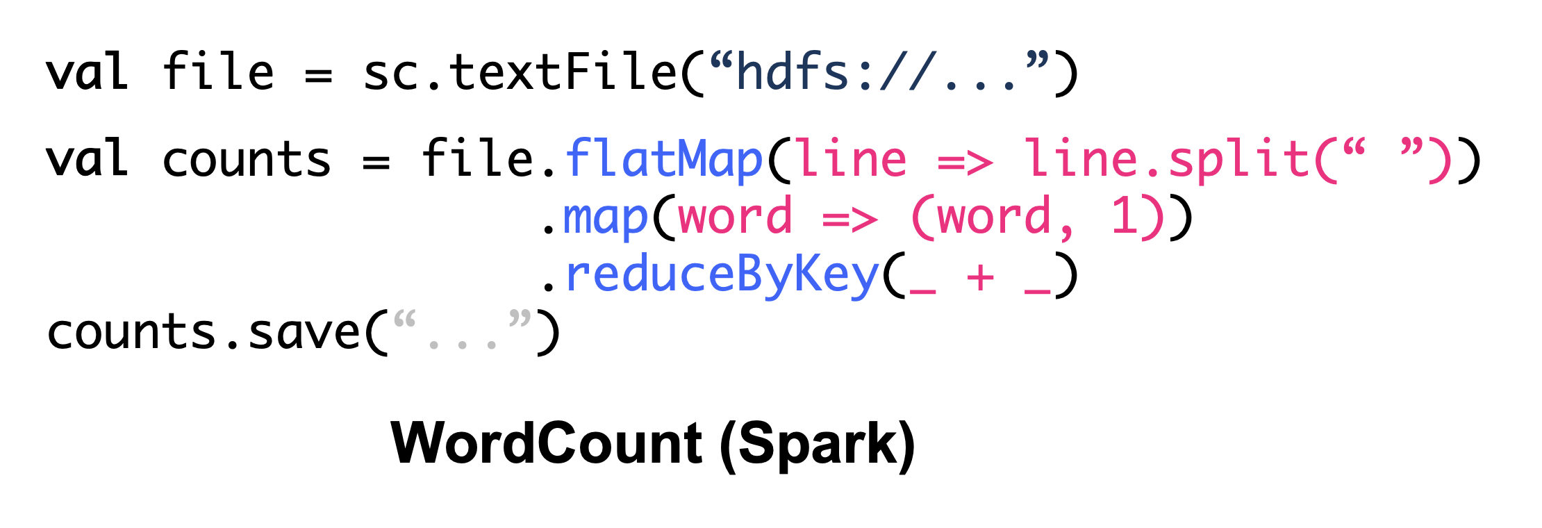
Spark

Motivation

Issues with Hadoop Mapreduce:

• Network and disk I/O costs: intermediate data has to be written to local disks and shuffled across machines, which is slow
• Not suitable for iterative (i.e. modifying small amounts of data repeatedly) processing, such as interactive workflows, as each individual step has to be modelled as a MapReduce job.

Spark stores most of its intermediate results in memory, making it much faster, especially for iterative processing

• When memory is insufficient, Spark spills to disk which requires disk I/O

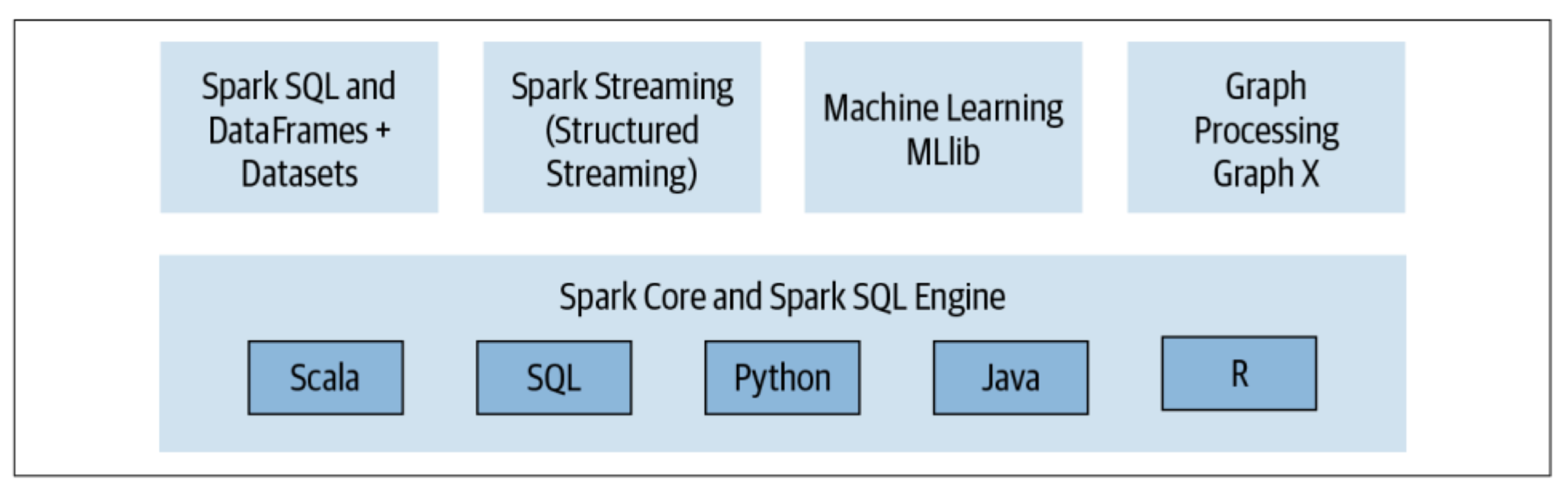
Spark components and API stack

Spark Architecture

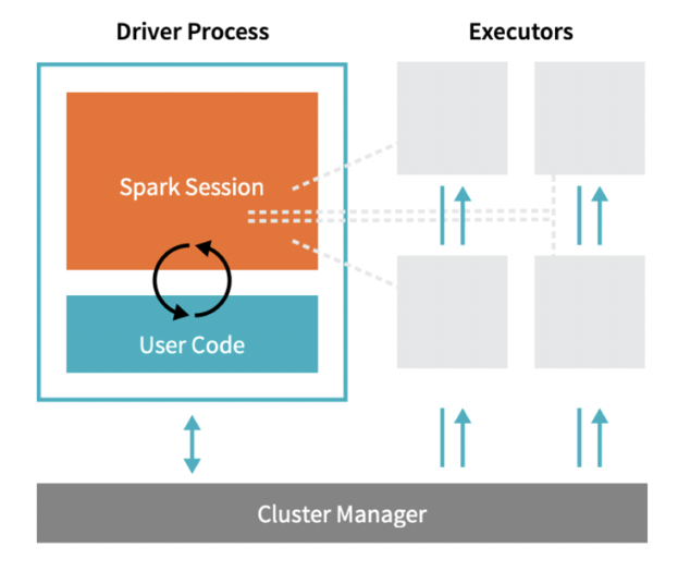
Driver Process responds to user input, manages the Spark application etc., and distributes work to Executors, which run the code assigned to them and send the results back to the driver

Cluster Manager (can be Spark’s standalone cluster manager, YARN, Mesos or Kubernetes) allocates resources when the application requests it

In local mode, all these processes run on the same machine

Spark APIs

Resilient Distributed Datasets (2011)

• A collection of JVM objects
• Functional operators (map, filter, etc)

DataFrame (2013)

• A collection of Row objects
• Expression-based operations
• Logical plans and optimizer

DataSet (2013)

• Internally ros, externally JVM objects
• Best of both worlds: type safe + fast

RDD

## Create an RDD of names, distributed over 3 partitions

dataRDD = sc.parallelize(["Alice", "Bob", "Carol", "Daniel"], 3) ## partition into 3 parts

RDDs are immutable, i.e. they cannot be changed once created.

This is an RDD with 4 strings. In actual hardware, it will be partitioned into the 3 workers.

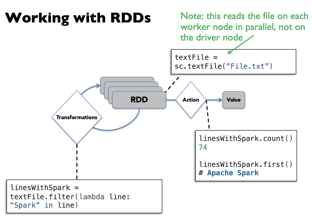
Transformations

Transformations are a way of transforming RDDs into RDDs.

nameLen = dataRDD.map(lambda s: len(s))

This represents the transformation that maps each string to its length, creating a new RDD. However, transformations are lazy. This means the transformation will not be executed yet, until an action is called on it

Advantages of being lazy: Spark can optimize the query plan to improve speed (e.g. removing unneeded operations)

• Examples of transformations: map, order, groupBy, filter, join, select

Actions

Actions trigger Spark to compute a result from a series of transformations.

## Asks Spark to retrieve all elements of the RDD to the driver node.
nameLen.collect() ## output: [5, 3, 5, 6]

Examples of actions: show, count, save, collect

Note

👉 RDDs are actually distributed across machines. Thus, the transformations and actions are executed in parallel. The results are only sent to the driver in the final step.

Caching

Log Mining example: Load error messages from a log into memory, then interactively search for various patterns

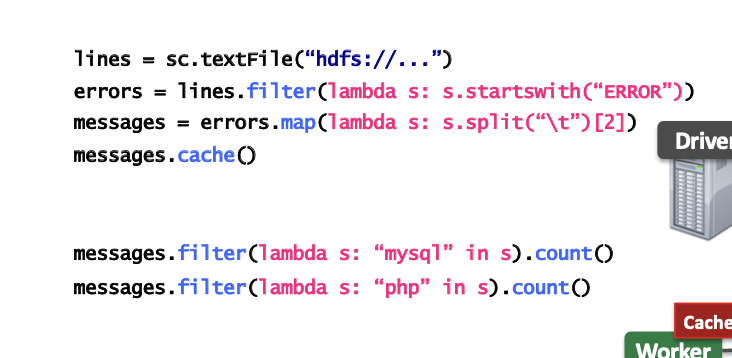
cache(): saves an RDD to memory (of each worker node).¢ persist(options): can be used to save an RDD to memory, disk, or off-heap memory (out-of-scope)

• When should we cache or not cache an RDD?
  • When it is expensive to compute and needs to be re-used multiple times.
  • If worker nodes have not enough memory, they will evict the “least recently used” RDDs. So, be aware of memory limitations when caching.

Directed Acyclic Graph (DAG)

Internally, Spark creates a graph (DAG) which represents all the RDD objects and how they will be transformed.

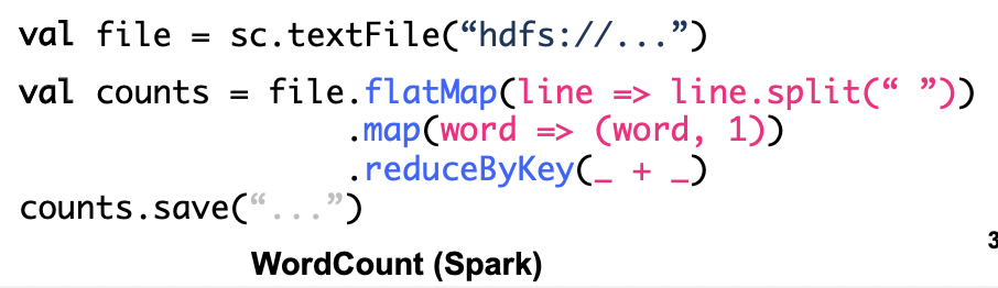
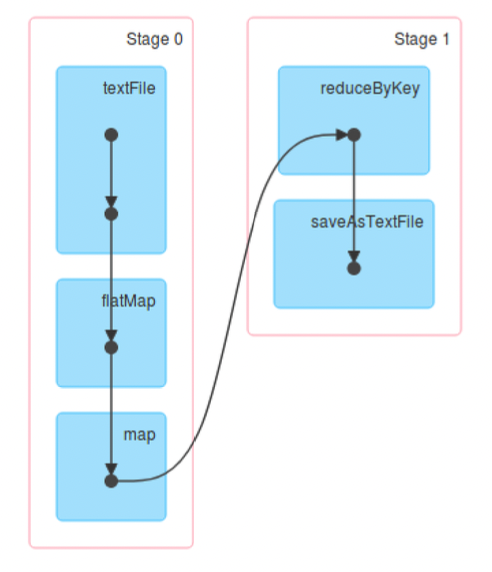
Narrow Dependencies: each partition of the parent RDD is used by at most 1 partition of the child RDD. E.g. map, flatMap, filter, contains

Wide dependencies: the opposite (each partition of parent RDD is used by multiple partitions of the child RDD). E.g. reduceByKey, groupBy, orderBy

In the DAG, consecutive narrow dependencies are grouped together as “stages”.

Within stages, Spark performs consecutive transformations on the same machines.

Across stages, data needs to be shuffled, i.e. exchanged across partitions, in a process very similar to map-reduce, which involves writing intermediate results to disk

Minimizing shuffling is good practice for improving performance.

Lineage and Fault Tolerance

Unlike Hadoop, Spark does not use replication to allow fault tolerance.

• Spark tries to store all the data in memory, not disk. Memory capacity is much more limited than disk, so simply duplicating all data is expensive.

Lineage approach: if a worker node goes down, we replace it by a new worker node, and use the graph (DAG) to recompute the data in the lost partition.

• Note that we only need to recompute the RDDs from the lost partition.

DataFrames

A DataFrame represents a table of data, similar to tables in SQL, or DataFrames in pandas.

Compared to RDDs, this is a higher level interface, e.g. it has transformations that resemble SQL operations.

• DataFrames (and Datasets) are the recommended interface for working with Spark - they are easier to use than RDDs and almost all tasks can be done with them, while only rarely using the RDD functions.
• However, all DataFrame operations are still ultimately compiled down to RDD operations by Spark.

flightData2015 = spark
  .read
  .option("inferSchema", "true")
  .option("header", "true").csv("/mnt/defg/flight-data/csv/2015-summary.csv")

flightData2015.sort("count").take(3) ## Sorts by ‘count’ and output the first 3 rows (action)
## output: Array([United States,Romania,15], [United States,Croatia...

flightData2015.createOrReplaceTempView("flight_data_2015")
maxSql = spark.sql("""
  SELECT DEST_COUNTRY_NAME, sum(count) as destination_total
  FROM flight_data_2015
  GROUP BY DEST_COUNTRY_NAME
  ORDER BY sum(count) DESC
  LIMIT 5
""")
maxSql.collect()

from pyspark.sql.functions import desc
flightData2015
  .groupBy("DEST_COUNTRY_NAME")
  .sum("count")
  .withColumnRenamed("sum(count)", "destination_total")
  .sort(desc("destination_total"))
  .limit(5)
  .collect()

DataSets

Datasets are similar to DataFrames, but are type-safe.

• In fact, in Spark (Scala), DataFrame is just an alias for DatasetRow]
• However, Datasets are not available in Python and R, since these are dynamically typed languages

case class Flight(DEST_COUNTRY_NAME: String, ORIGIN_COUNTRY_NAME: String, count: BigInt)
val flightsDF = spark.read.parquet("/mnt/defg/flight-data/parquet/2010-summary.parquet/")
val flights = flightsDF.as[Flight]
flights.collect() // return objects of the “Flight” class, instead of rows.

Supervised ML Basics

Typical ML Pipeline

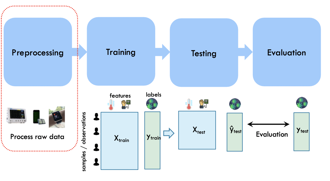
Data preprocessing

Data quality

Why is data missing?

• ­Information was not collected: e.g. people decline to give weight
• Missing at random: missing values are randomly distributed. If data is instead missing not at random: then the missingness itself may be important information.

How to handle missing values?

• Eliminate objects (rows) with missing values
• Or: fill in the missing values (“imputation”)
  • E.g. based on the mean / median of that attribute
  • Or: by fitting a regression model to predict that attribute given other attributes
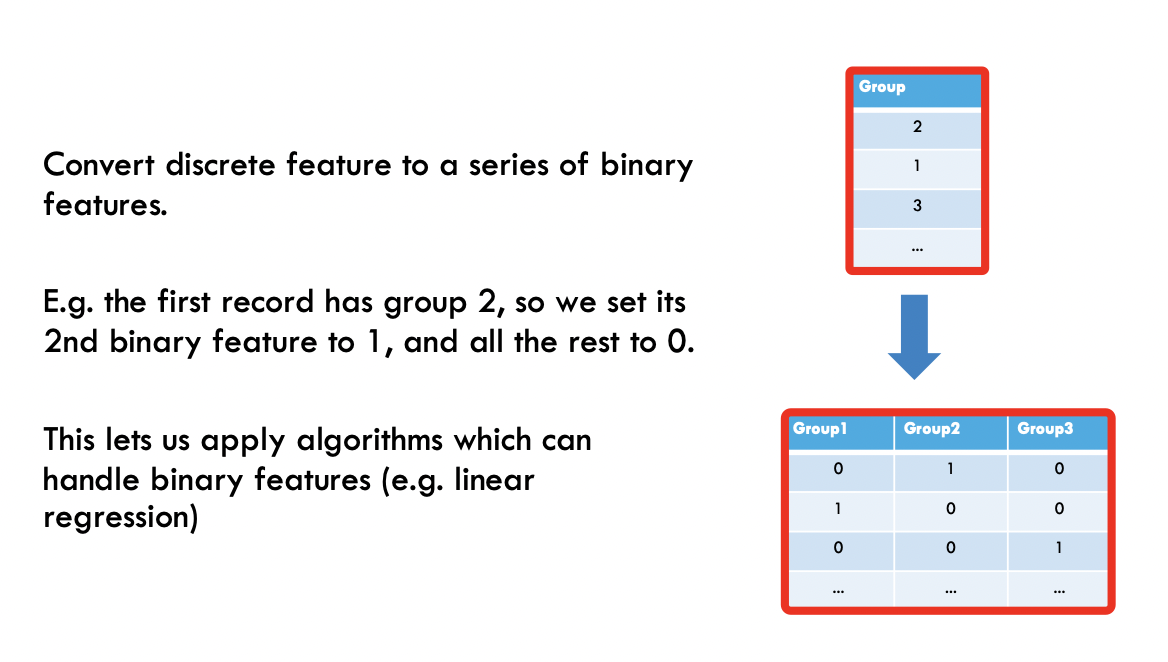
  • Dummy variables: optionally insert a column which is 1 if the variable was missing, and 0 otherwise

One hot encoding

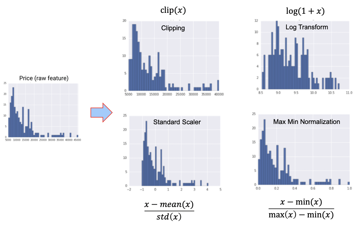
Normalization

Training and Testing

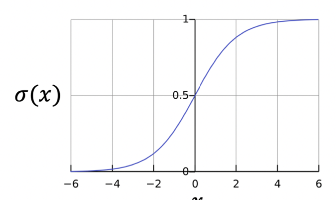
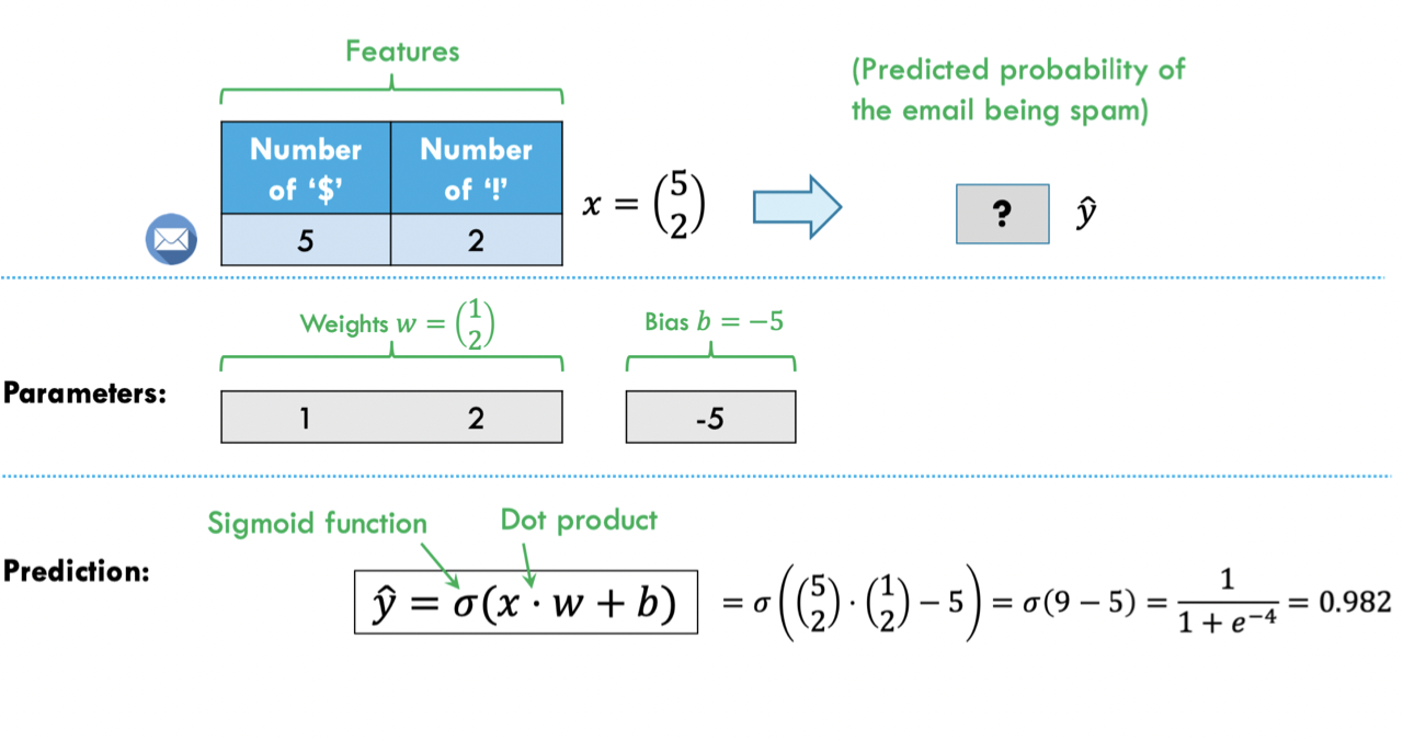
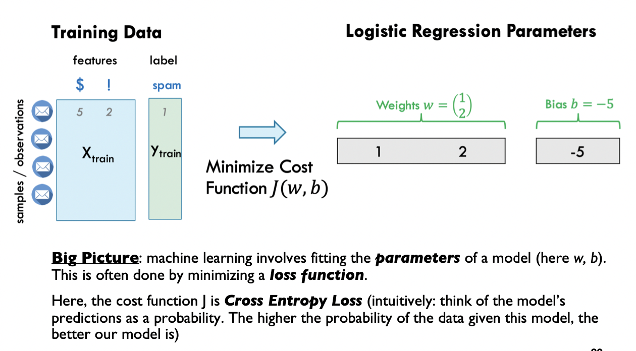
Logistic Regression

Sigmoid function:

$$\sigma(x) = \frac{1}{1 + e^{-x}}$$

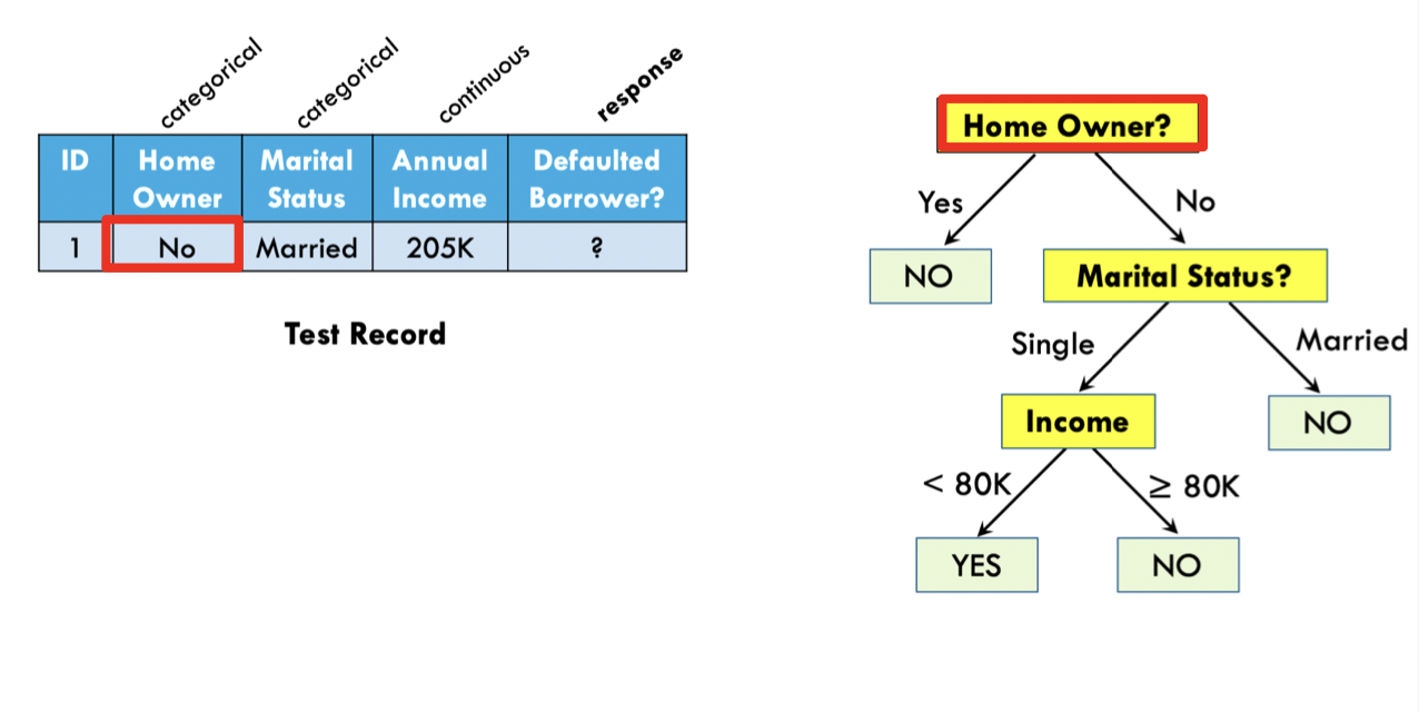
Decision Trees

Random Forests and Gradient Boosted Trees

Decision trees are simple, interpretable and fast, but suffer from poor accuracy, and are not robust to small changes

• For applications where interpretability is especially important, learning “optimal decision trees” is still an active area of research

Random Forests and Gradient Boosted Trees are very popular approaches which combine a large number of decision trees

On tabular data, their accuracy is still highly competitive with neural networks, and are faster, easier to tune, and more interpretable

Evaluation

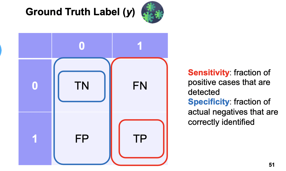
Accuracy: fraction of correct predictions (TN and TP)

Sensitivity: fraction of positive cases that are detected

Specificity: fraction of actual negatives that are correctly identified

Spark MLLib

Simple logistic regression model

from pyspark.ml.classification import LogisticRegression

training = spark.read.format("libsvm").load("data/mllib/sample_libsvm_data.txt")
lr = LogisticRegression(maxIter=10)
lrModel = lr.fit(training)

print("Coefficients: " + str(lrModel.coefficients))
print("Intercept: " + str(lrModel.intercept))

Pipelines

Transformers

Transformers are for mapping DataFrames to DataFrames

• Examples: one-hot encoding, tokenization
• Specifically, a Transformer object has a transform() method, which performs its transformation

Generally, these transformers output a new DataFrame which append their result to the original DataFrame.

• Similarly, a fitted model (e.g. logistic regression) is a Transformer that transforms a DataFrame into one with the predictions appended.

Estimators

Estimator is an algorithm which takes in data, and outputs a fitted model. For example, a learning algorithm (the LogisticRegression object) can be fit to data, producing the trained logistic regression model.

They have a fit() method, which returns a Transformer

Training time

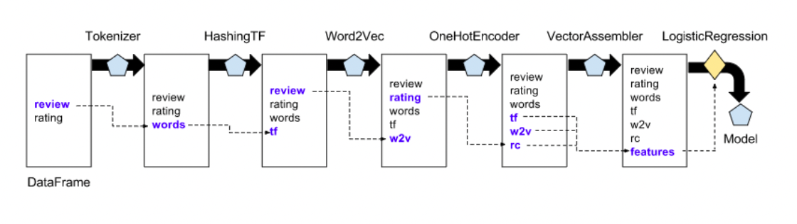
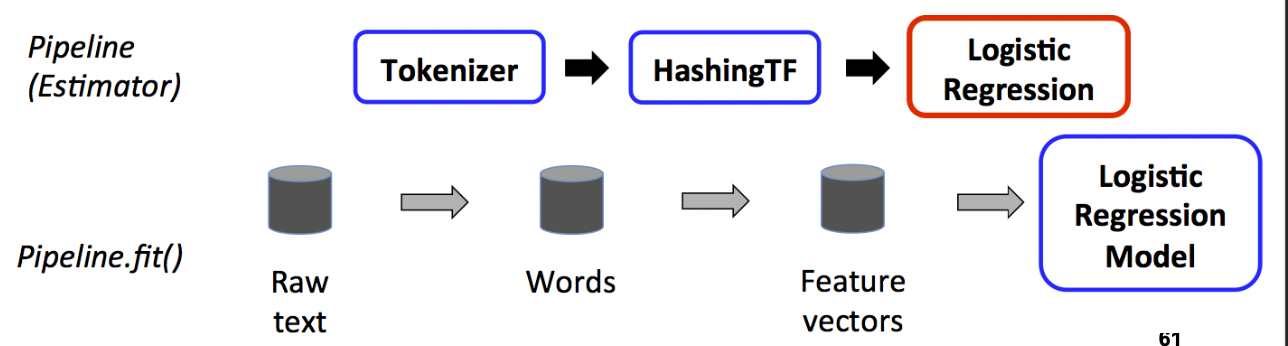
A pipeline chains together multiple Transformers and Estimators to form an ML workflow.

It is an Estimator. When Pipeline.fit() is called:

• Starting from the beginning of the pipeline:
• For Transformers, it calls transform()
• For Estimators, it calls fit() to fit the data, then transform() on the fitted model

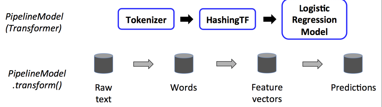
Test time

The output of Pipeline.fit() is the estimated pipeline model (of type PipelineModel).

• It is a transformer, and consists of a series of Transformers.
• When its transform() is called, each stage’s transform() method is called.

Example

training = spark.createDataFrame([
  (0, "a b c d e spark", 1.0), (1, "b d", 0.0),
  (2, "spark f g h", 1.0),
  (3, "hadoop mapreduce", 0.0)
], ["id", "text", "label"])

## Configure an ML pipeline, which consists of three stages: tokenizer, hashingTF, and lr.
tokenizer = Tokenizer(inputCol="text", outputCol="words")
hashingTF = HashingTF(inputCol=tokenizer.getOutputCol(), outputCol="features")
lr = LogisticRegression(maxIter=10, regParam=0.001)
pipeline = Pipeline(stages=[tokenizer, hashingTF, lr])

## Fit the pipeline to training documents.
model = pipeline.fit(training)

Simplified PageRank

Flow Model

Define a “rank” or importance $r_j$ **for page j

$$r_j = \sum_{i \rarr j}{\frac{r_i}{d_i}}$$

where $d_i$ = number of out-links of node i (out-degree)

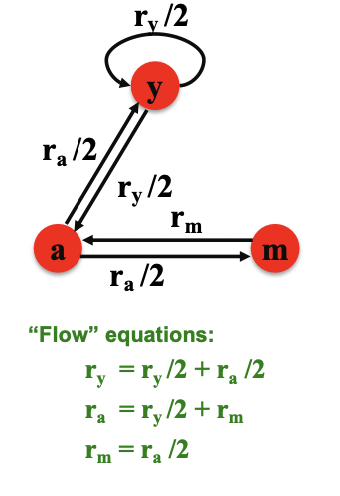
3 equations, 3 unknowns, 1 redundant equation

• No unique solution
• All solutions are rescalings of each other

Additional contraint: $r_y + r_a + r_m = 1$

Solution: $r_y=r_a=0.4, r_m=0.2$

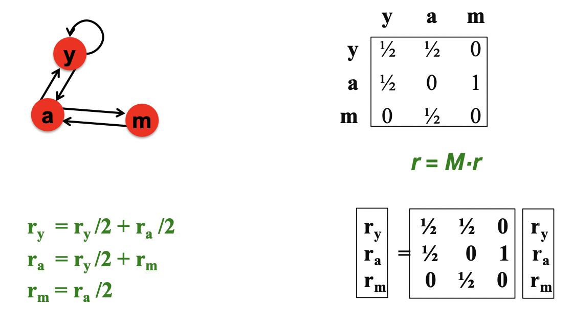
Matrix Formulation

Stochastic adjacency matrix $M$: page i has $d_i$ out-links, if $i \rarr j$, then $M_{ji} = \frac{1}{d_i}$ else $M_{ji}=0$

• M is a column stochastic matrix (columns sum to 1)

Rank vector $r$: $r_i$ is the importance score of page i, and $\sum_i{r_i} = 1$

The flow equation can be written as

$$r = M \cdot r$$

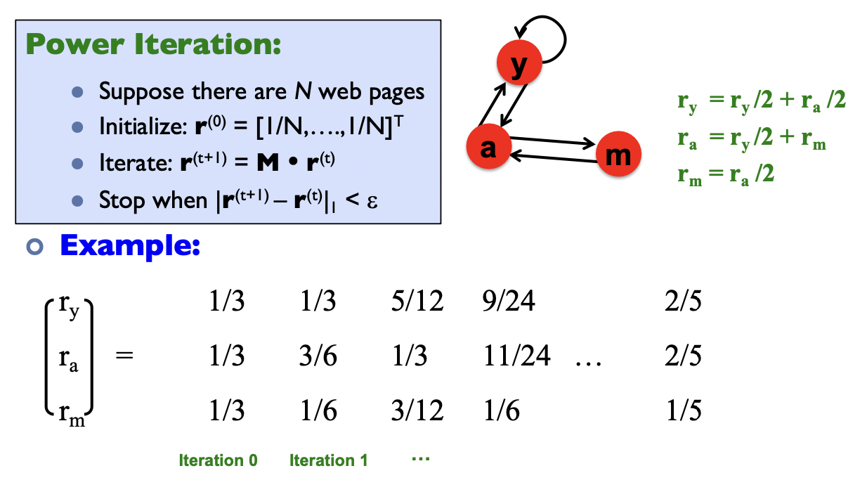
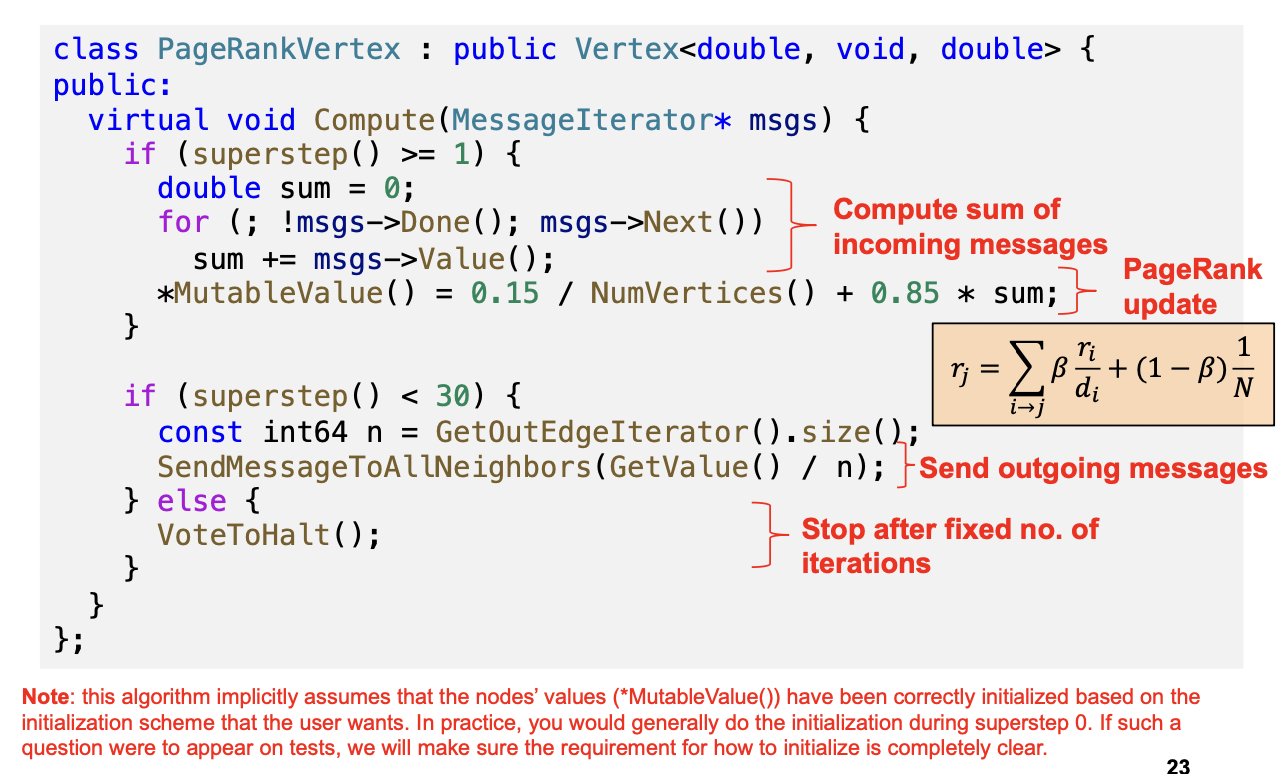
Power iteration method

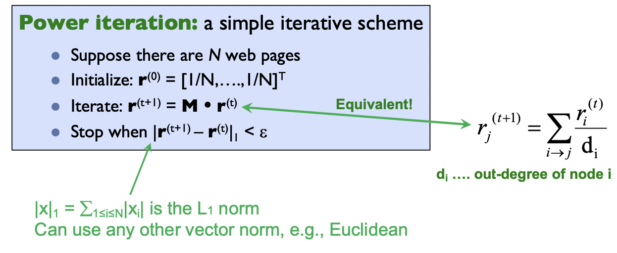
Intuitive interpretation of power iteration: each node starts with equal importance (of 1/N). During each step, each node passes its current importance along its outgoing edges, to its neighbors.

Random walk interpretation

Imagine a random web surfer:

• At time t = 0, surfer starts on a random page
• At any time t, surfer is on some page i
• At time t + 1, the surfer follows an out-link from i uniformly at random
• Process repeats indefinitely

Let:

• $p(t)$ … vector whose $i^{th}$ coordinate is the prob. that the surfer is at page ” at time t
• So, $p(t)$ is a probability distribution over pages

Stationary Distribution: as $t \rarr \infin$, the probability distribution approaches av‘steady state’ representing the long termvprobability that the random walker is at each node, which are the PageRank scores

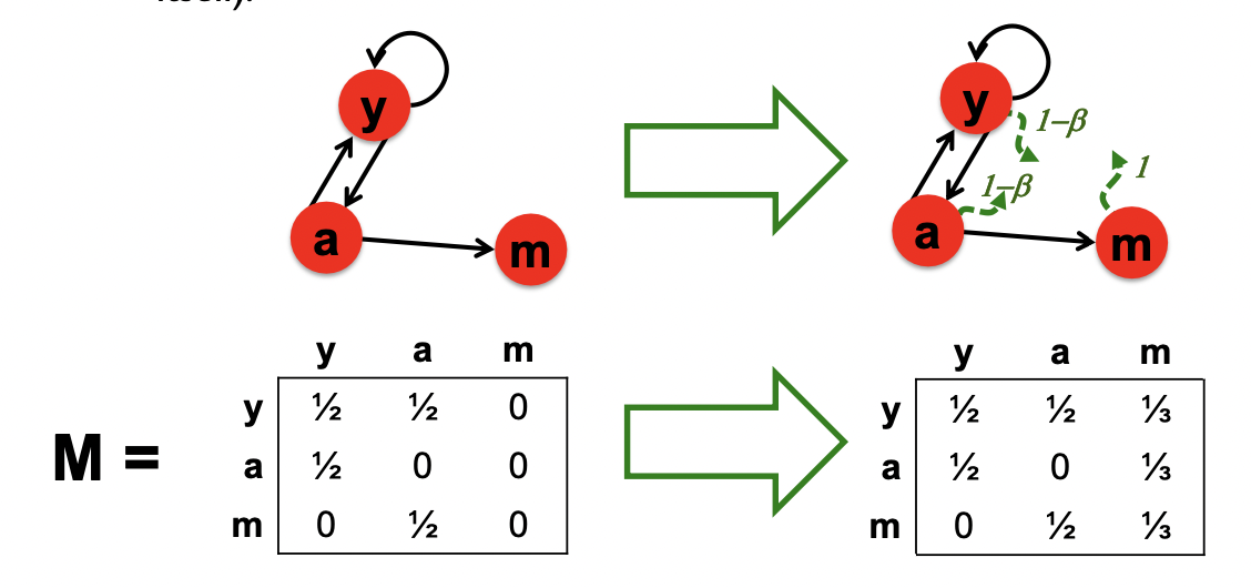
PageRank (with teleports)

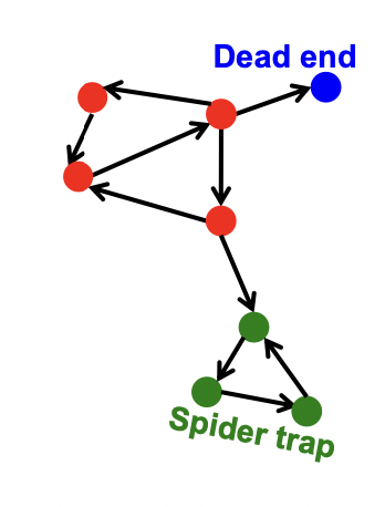
Some pages are dead ends (have no out-links)

• Random walk has “nowhere” to go to
• Such pages cause importance to “leak out”

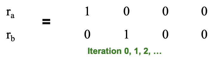
Spider traps (all out-links are within the group)

• Random walk gets “stuck” in a trap
• And eventually spider traps absorb all importance

Teleports

The Google solution for spider traps: At each time step, the random surfer has two options

• With prob. b, follow a link at random
• With prob. 1-b, jump to some random page
• Common values for b are in the range 0.8 to 0.9

If at a Dead End, Always Teleport

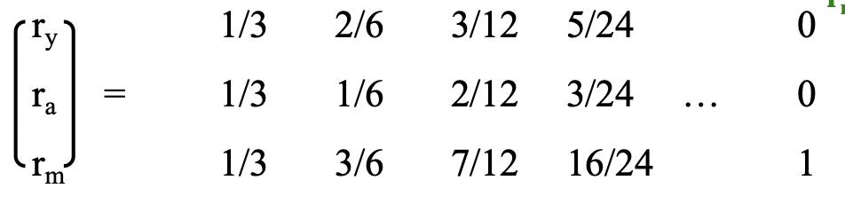
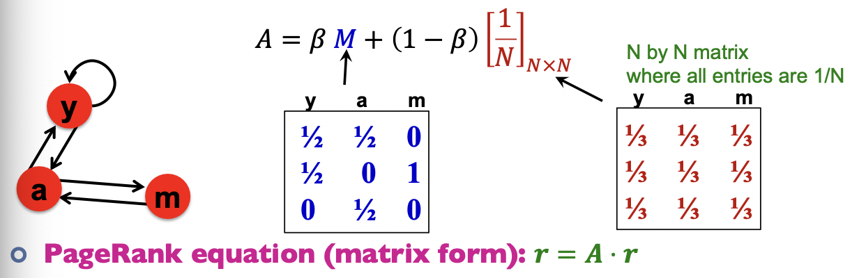
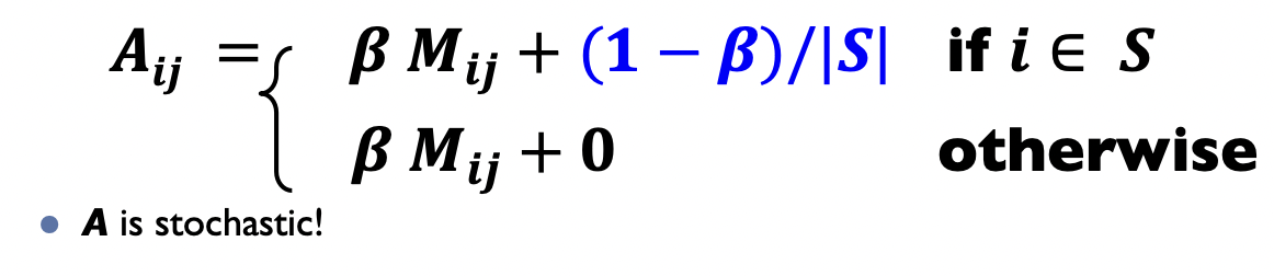
PageRank equation

$$r_j = \sum_{i\rarr j}{\beta\frac{r_i}{d_i} + (1 - \beta)\frac 1 N}$$

The Google matrix

$$A = \beta M + (1-\beta) \left[\frac 1 N \right]_{N\times N}$$

Topic-specific PageRank

Goal: Evaluate Web pages not just according to their popularity, but by how close they are to a particular topic, e.g. “sports” or “history”

Standard PageRank: Teleport can go to any page with equal probability

Topic Specific PageRank: Teleport can go to a topic-specific set of “relevant” pages (teleport set)

Pregel

Computational Model

Computation consists of a series of supersteps

In each superstep, the framework invokes a user-defined function, compute(), for each vertex (conceptually in parallel)

compute() specifies behavior at a single vertex v and a superstep s:

• It can read messages sent to v in superstep s -1;
• It can send messages to other vertices that will be read in superstep s + 1;
• It can read or write the value of v and the value of its outgoing edges (or even add or remove edges)

Termination:

• A vertex can choose to deactivate itself
• Is “woken up” if new messages received
• Computation halts when all vertices are inactive

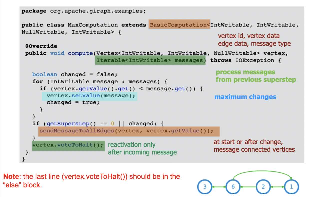
Example: Computing max

Compute(v, messages):
  changed = False
  for m in messages:
    if v.getValue() < m:
      v.setValue(m)
      changed = True
  if changed:
    for each outneighbor w:
      sendMessage(w, v.getValue())
  else:
    voteToHalt()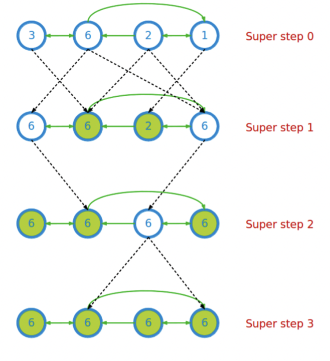

Implementation

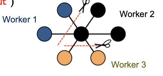
Master & workers architecture

• Vertices are hash partitioned (by default) and assigned to workers
• Each worker maintains the state of its portion of the graph in memory
• Computations happen in memory
• In each superstep, each worker loops through its vertices and executes compute()
• Messages from vertices are sent, either to vertices on the same worker, or to vertices on different workers (buffered locally and sent as a batch to reduce network traffic)

Fault tolerance

• Checkpointing to persistent storage
• Failure detected through heartbeats; corrupt workers are reassigned and reloaded from checkpoints

Giraph architecture

• Giraph originated as the open-source counterpart to Pregel, with several features beyond the basic Pregel model.
• Employs Hadoop’s Map phase to run computations
• Employs ZooKeeper (service that provides distributed synchronization) to enforce barrier waits

PageRank in Pregel

Stream

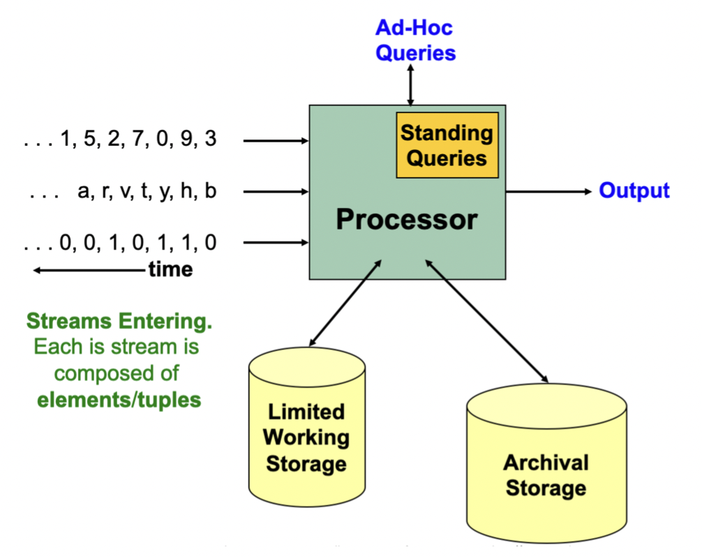
Reservoir Sampling

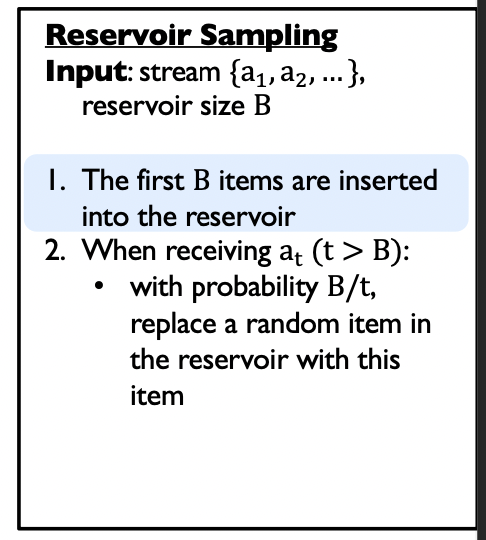
Given: a stream of items ${ a_1, a_2, \dots }$

Goal: maintain a ‘uniform random sample**’** of fixed size B over time

Stream Data Processing System: Storm

Tuple: an ordered list of named values, like a database row

• Items in a tuple can be accessed either via their index, or their name

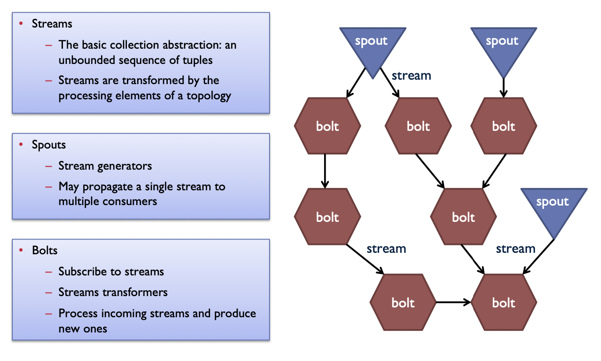
To do computation in Storm, the user creates a topology, which is a computation graph

• Nodes hold processing logic (i.e., transformation over its input)
• Edges indicate communication between nodes
• Each topology corresponds to a Storm job. Once started, a job continues running forever until killed.

Storm architecture

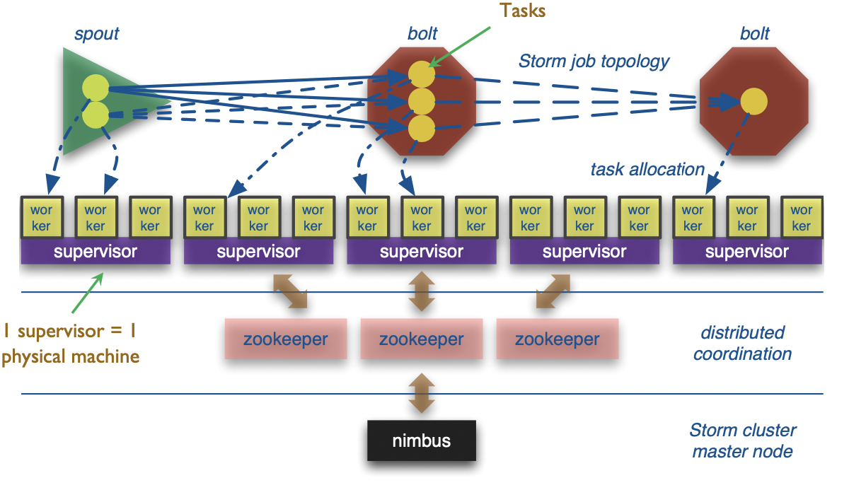
Bolts are executed by multiple executors in parallel, called “tasks”

Stream groupings:

• Shuffle grouping: tuples are randomly distributed across tasks
• Field grouping: based on the value of a (user-specified) field
• All: replicate tuple across all tasks of the target bolt